Quantum Espresso Performance Report
Test Submission
A test submission of https://github.com/ukri-bench/benchmark-quantumespresso.
This is not a commentary on code quality, but an indicator of the quality of the current SHAREing testing methodology as of this date.
Aim
- Provide a test of the submission forms
- Provide feedback on the performance workbook, link to the performance workbook as of 13.01.2026
Section 3.1, Benchmark setup
The benchmarks are provided with separate setup and run commands.
spack install quantum-espresso@7.4.1+openmp+mpi+scalapack

mpirun -np <number of processors> pw.x -i <input file> > <output file>
../../bin/extract.py <output file>
For example:
spack install quantum-espresso@7.4.1+openmp+mpi+scalapack


cd benchmarks/ausurf/


mpirun -np 10 pw.x -i ausurf.in  > ausurf.out
../../bin/extract.py ausurf.out
There are not simple scaling parameters available in the input to these benchmarks.
The number of atoms and the structure size are dependent on the material to be modelled, and would give nonphysical results if changed.
This problem has non trivial scaling of workload.
Scaling is presented in DOI 10.1088/0953-8984/21/39/395502, Figure. 3 for 32 processors to 512, as referenced on the Quantum Espresso website. This is for a fixed simulation size. More benchmarks are collated in a github repository provided by the Quantum Espresso team.
3.2 Description of working environment
1. Hamilton/Bede
    a. `multi` queue for requestng whole nodes (to reduce timing noise from other programs)
    b. Limited to one node, 2 GPU's as part of testing submission
2. Assessment tools
    a. High level assessment
            i. wall time
            ii. self reported stats from quantum-espresso regarding cpu/gpu times.
    b. low level assessment (requires privileges on host)
        i.CPU wait time (for I/O / heterogenous compute)
        ii.cache
        iii.memory accesses
        iv. LIKWID to access performance counters, topology etc. # 3.3 Compiler Setup
Built with Spack
- Spack in the default configuration does not use any cpp,cxx of fortran flags.
- Using the nvhpc patch triggers -O3 and -fast flags for the fortran compiler.
- spack spec : quantum-espresso%nvhpc + cuda.
Alter Spack configuration to include -O3 as a default.
Spack is configured to be aware of the available CPU feature sets on build (for example, for Hamilton with default compilation - {“target”:{“name”:”zen”,”vendor”:”AuthenticAMD”,”features”:[“abm”,”aes”,”avx”,”avx2”,”bmi1”,”bmi2”,”clflushopt”,”clzero”,”cx16”,”f16c”,”fma”,”fsgsbase”,”lahf_lm”,”mmx”,”movbe”,”pclmulqdq”,”popcnt”,”rdseed”,”sse”,”sse2”,”sse3”,”sse4_1”,”sse4_2”,”sse4a”,”ssse3”,”xsave”,”xsavec”,”xsaveopt”]}. It is unclear if this is being taken advantage of.
MAQAO should present missed compiler optimisation opportunities.
Increasing optimisation level may require the system to be reconverged to confirm accuracy. This may be outside of the scope of the assessment.
3.4 Code Complexity
TDDFT is polynomial in time, atoms and electrons.Computational complexity of time-dependent density functional theory
In traditional DFT, computation time grows with O(Syste size^3), and while techniques empllyed in large system scale DFT codes can reduce this to closer to a linear scaling, it should be assumed quantum-espresso scales in this way. It can be reasoned that the memory requirements for DFT must also scale worse than linearly, as the density functional alone is linearly dependent on system size.
Load balancing for molecular integration is best performed heuristically, so it is likely changes to the shape of the underlying hardware assignment could cause irregularities in scaling behaviour.
3.5: Memory, Storage and I/O
Memory is reported at approx 23GB for the ausurf benchmarks.
Generates ~3.6GB of output files in #OUTDIR#
3.6: Hardware information
AMD EPYC 7702 64-Core Processor on 1 node - Hamilton.
processor       : 0-63
model name      : AMD EPYC 7702 64-Core Processor

MemTotal:       263152912 kB   #~250GB per node
MemFree:        256995420 kB
MemAvailable:   258291956 kB
GPU:
- NVIDIA H200 NVL, each with 144GB
3.7 Code separation
Requires domain knowledge of quantum-espresso to identify science producing sections of code, vs compatibility, safety etc sections.
3.8 Historic optimisations
Requires domain knowledge of quantum-espresso to identify algorithmic optimistions vs poorly implemented (i.e. confusing or non-functinoal) or justified (i.e. not valid for hardware in use, not valid fo majority test cases) computational justifications.
Software details (in progress!)
We recommend the analyst provide key pieces of information (which currently contains dummy info):
- Program name - Quantum Espresso
- Parallel model (e.g., OpenMP, MPI, etc.) - Serial, OpenMP and MPI, MPI and GPU
- Compiler (including optimisation flags) - cmake build type “Release”, gcc Ofast, built with spack install quantum-esppresso@7.5%nvhpc +cuda
- Libraries/dependencies - mpi, nvcc
- Details on data input - using the ausurf benchmark configuration
Report
High Level Analysis
from topics.core import core_perf
from topics.intra_node import intra_node_perf
from topics.inter_node import inter_node_perf
from topics.gpu import gpu_perf
from topics.io import io_perf
from topics.summary import summary_perf
Core
For a high-level core analysis we just want 2 measurements for a serial code:
- Maximum peak performance (Mflops/s)
- Measured average peak FLOPS (Mflops/s)
FLOPS
To measure these we use LIKWID, i.e., for FLOPS we use
likwid-bench -t peakflops -W S0:16kB:1
likwid-perfctr -f -C 0 -g FLOPS_DP ./my_exe
in which the input data for the peakflops microbenchmark is half the L1 cache.
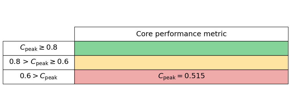
# Target peak per core (Mflops/s)
maximum_performance = 8825.70
# Measured average application peak (Mflops/s)
measured_performance = 4541.7572
We read these values into our core_perf class
core_performance_stats = core_perf(maximum_performance, measured_performance)
Generate the core performance table below
core_performance_stats.core_perf_table()
Intra-node
To quantify intra-node performance at a high level we reply simply on runtimes under a strong scaling analysis.
Serial run
If possible, we first measure the runtime of a serial application without any parallel libraries, e.g., compile without the -fopenmp flag. This can seem redundant but allows us to see the overhead of the parallel library when compared to a single-core run including the parallel library.
If the parallel library cannot be switched off simply, then we suggest just setting the serial runtime equal to a single-core (with parallel library enabled) runtime.
Strong scaling
We now perform a strong scaling analysis by keeping our problem sized fixed but increasing the core count up to the maximum for your hardware. For an OpenMP code the thread number can be set simply with the OMP_NUM_THREADS environment variable, however, with this method thread affinity can be an issue. It can make performance variable relative to a thread pinned run.
Thread pinning can be easily acheived by setting the OMP_PROC_BIND environment variable to close, however, we again make use of LIKWID
likwid-pin -c N:0-3 ./my_exe
This command can be nested into a for loop to increase the core count to efficiently perform a strong scaling analysis.
Input data
In the cell below we ask for the:
- Serial runtime
- A list of the core numbers used for the strong scaling
- A list of the relative runtime per number of cores
# Enter serial performance time (s)
import numpy as np
serial_time = 3714.0

data = np.array([(32,252.24),(16,413.00),(8,708.36),(4,1327.05),(2,2288.44 ),(1,3714.0)
],dtype=[('Core count', 'i4'),('Loop Time','f4')])

# enter number of cores in each trial
number_of_cores = data['Core count']

# Enter time for each number of cores (s)
time = data['Loop Time']
We read these values into our intra_node_perf class
intra_node_performance_stats= intra_node_perf(serial_time, number_of_cores, time)
[0.46012726 0.56204599 0.6553871  0.69967216 0.81146985 1.        ]
[8 4]
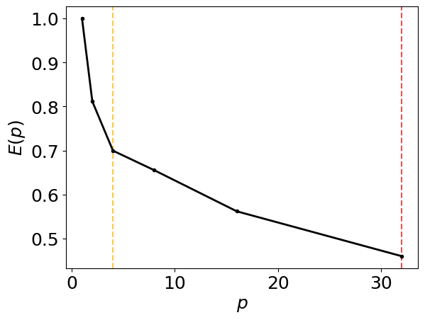
Generate the intra-node parallel efficiency plot below, including amber and red vertical lines which indicate the core counts below which the parallel efficiency drops to 80% and 60%, respectively.
intra_node_performance_stats.parallel_efficiency_figure()
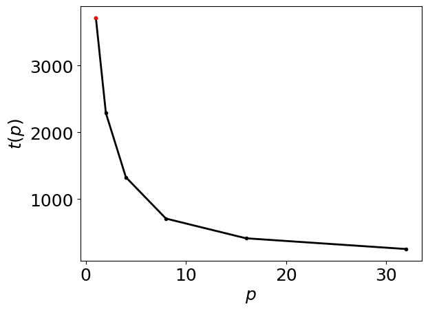
Generate the intra-node runtimes plot below
intra_node_performance_stats.runtimes_figure()
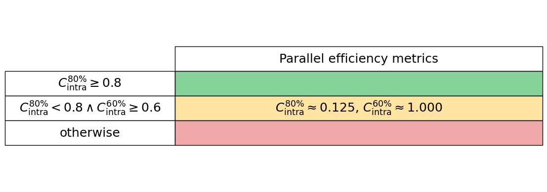
Generate the intra-node performance table below
intra_node_performance_stats.intra_node_perf_table()
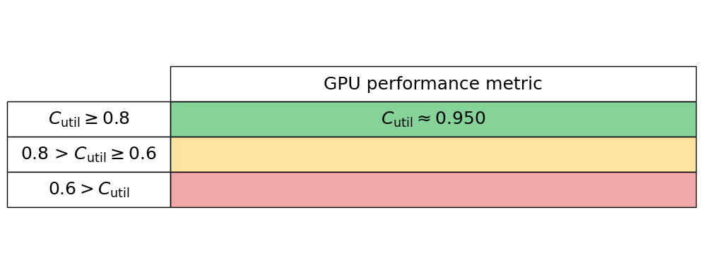
GPU
To quantify GPU performance at a high level we use two metrics:
- GPU utilisation or occupancy
- GPU memory usage
GPU utilisation or occupancy
This metric is typically a measure of the proportion of computational resources in use by the code. In Nvidia language this will likely be the proportion of streaming multiprocessors in use. We simply read this metric into our gpu_perf class below, and most GPU vendor’s tools will give this high-level metric for their hardware.
GPU memory usage
We compute the proportion of the maximum memory footprint used by the software by reading the theoretical gpu_peak_memory (typically from the vendor’s data sheets) and measure the actual memory usage, gpu_measured_memory, which again is typically given from most vendor tools.
gpu_runtime_data = np.array([(1,67.18),(2,41,35)
],dtype=[('GPU count', 'i4'),('Loop Time','f4')])
#gpu used for 15.61+17.68+4.5 total seconds
gpu_time_ratio = (15.61 + 17.68 + 4.5)/gpu_runtime_data["Loop Time"][0]
print("GPU run time ratio:",gpu_time_ratio)
GPU run time ratio: 0.5625186041728631
We read these values into our gpu_perf class
gpu_performance_stats = gpu_perf(gpu_utilisation)
Generate the GPU performance table below
gpu_performance_stats.gpu_perf_table()
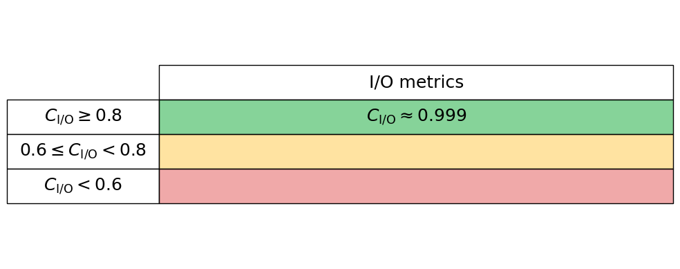
I/O
To quantify I/O (Input/Output) performance at a high level we simply ask what proportion of an applications total runtime is spent in read and writes. Many performance tools can give these high-level metrics, e.g., Intel VTune and Linaro Performance Reports. Typically these measures are given for both reads and writes separately, so we here read these two proportions in independently, thus the performance is charactertised by $C_{\mathrm{I/O}} = 1 - (C_{\mathrm{read}} + C_{\mathrm{write}})$. Therefore a low $C_{\mathrm{I/O}}$ value implies that the application is spending significant time in reading and writing to disk.
read_proportion = 0.00
write_proportion = 0.00728
We read these values into our io_perf class
io_performance_stats = io_perf(write_proportion, read_proportion)
Generate the I/O performance table below
io_performance_stats.io_perf_table()
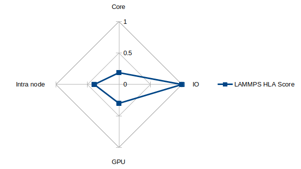
High level summary
The intra node performance degrades quickly for this problem set, with less than 40% of the parallel efficiency reached before 32 cores. The GPU performance is massively improved, with a single Nvidia H200 outperforming 32 cores by a factor of more than 3 when measuring runtime. This is despite the fact that only 56% of the total runtime had the GPU utilised for this problem. The memory utilisation of the GPU’s vram was low, but given the problem size this is to expected. The CPU and GPU versions of the code are not unified at present, with unification planned as detailed in the project roadmap. The total memory required for these test simulations was well below the single node capacity on Hamilton. Key regions of development are OpenMP performance; GPU performance and benchmarking of different hardware types; improving building and packaging; interfacing with scripting languages and improving pseudopotential support. IO can be relatively concise for a given compute size so the IO measurements presented here being a small fraction of total runtime was expected.
Low level analysis
This project has received funding through the UKRI Digital Research Infrastructure Programme under grant UKRI1801 (SHAREing)