HemeLB Performance Report

A test submission of HemeLB, available on the HemeLB GitHub repository master branch.

Disclaimers

1. This is not a commentary on code quality, but an indicator of the quality of the current SHAREing testing methodology as of this date, 20/03/26.
2. This forms only a preliminary assessment of submission suitability and does not guarantee a full assessment. The pre-assesment will be provided to the submitter with information on how to continue to assessment or rejection.

Preassessment Overview

• 1: Code
• 2: Description of working environment
• 3: Building
• 4: Running
• 5: Code complexity
• 6: I/O
• 7: Assessment structure

1: Code

The main codebase for HemeLB can be cloned with

git clone https://github.com/UCL-CCS/HemePure.git

We use the master branch for analysis.

2: Description of working environment

Here we describe some details of the system we will be running on and how we are configuring the software environment.

2.1: Hardware information

We run on Hamilton, one of the HPC clusters hosted at Durham University. There are 120 standard compute nodes and 2 high-memory ones:

Specification	Per node
Processors	2x AMD EPYC 7702 64-Core Processor
Clock	3289.415MHz
Sockets	2
Cores	128
RAM	Standard: 256GB (246GB available to users) High-memory: 2TB
Local storage	400GB SSD

Each socket on each compute node is divided into 4 NUMA domains that each have a dedicated memory channel. Each of these NUMA domains are further split into 4 groups, where each has its own 16MB L3 cache (totalling to 256MB in one processor). Each of these groups contains 4 core that each have 512KB of L2 cache and 32KB of L1 cache.

2.2: Dependencies

We require a C compiler, MPI library and CMake for building

module load gcc openmpi cmake

Giving an environmental setup of:

Currently Loaded Modulefiles:
  1) gcc/11.2        2) openmpi/4.1.1   3) cmake/3.18.4

We also do not have to manually set any environment variables or add any paths.

3: Building

The build scheme is split into two phases: building dependencies then building the source code, listed below.

Dependency build

1. Create dep/build/ directory and cd into it
2. In this directory run ccmake -B. -H../ and press c to configure then e to exit
3. Then back at the command line configure with CMake using

   cmake -DCMAKE_C_COMPILER=gcc \
      -DCMAKE_CXX_COMPILER=g++ \
      -DCMAKE_CXX_FLAGS="-g" \
      -DHEMELB_COMPUTE_ARCHITECTURE=NEUTRAL \
      -DCMAKE_CXX_EXTENSIONS=OFF \
      -DHEMELB_USE_VELOCITY_WEIGHTS_FILE=ON \
      -DHEMELB_INLET_BOUNDARY=LADDIOLET \
      -DHEMELB_WALL_INLET_BOUNDARY=LADDIOLETSBB \
      -DHEMELB_OUTLET_BOUNDARY=NASHZEROTHORDERPRESSUREIOLET \
      -DHEMELB_WALL_OUTLET_BOUNDARY=NASHZEROTHORDERPRESSURESBB \
      -DHEMELB_LOG_LEVEL="Info" \
      -DHEMELB_USE_MPI_PARALLEL_IO=OFF \
      -DCMAKE_BUILD_TYPE=Release \
      ..
   

4. Then run make in dep/build/

Source code build

1. Create src/build/ directory and cd into it
2. In this directory run ccmake -B. -H../ and again press c to configure and then e to exit
3. Then back at the command line configure with CMake using

   cmake -DCMAKE_C_COMPILER=gcc \ 
      -DCMAKE_CXX_COMPILER=g++ \
      -DCMAKE_CXX_FLAGS="-g" \
      -DHEMELB_COMPUTE_ARCHITECTURE=NEUTRAL \
      -DCMAKE_CXX_EXTENSIONS=OFF \
      -DHEMELB_USE_VELOCITY_WEIGHTS_FILE=ON \
      -DHEMELB_INLET_BOUNDARY=LADDIOLET \
      -DHEMELB_WALL_INLET_BOUNDARY=LADDIOLETSBB \
      -DHEMELB_OUTLET_BOUNDARY=NASHZEROTHORDERPRESSUREIOLET \
      -DHEMELB_WALL_OUTLET_BOUNDARY=NASHZEROTHORDERPRESSURESBB \
      -DHEMELB_LOG_LEVEL="Info" \
      -DHEMELB_USE_MPI_PARALLEL_IO=OFF \
      -DCMAKE_BUILD_TYPE=Release \
      ..
   

4. Run make in src/build/

4: Running

With the build instructions documented, we now run through the necessary information for running the code.

4.1: Data

The code requires input data which is hosted on Zenodo. Here we chose the test data in TestPipe.tar.gz, in particular the /nobackup/<username>/NVIDIA-TestPipe/input_VP.xml input file.

4.2: Runtime commands

mpirun -np xx hemepure -in input.xml -out results

where input.xml is the file in the path: /nobackup/<username>/NVIDIA-TestPipe/input_VP.xml.

It should be noted that by default HemeLB can run across a minimum of 3 cores, i.e., there is no serial implementation. This impacts how we perform our core and intranode analyses, though these points will be discussed further in the high-level analysis below.

5: Code Complexity

Next to no scaling information is given in the documentation. There are input files given to generate a weak scaling, though we do not yet include that in the analysis here as the internode analysis is still under development.

6: Memory, Storage and I/O

For the TestPipe examples the peak memory consumption given by the sacct command is approximately 17.6GB. The storage for the input files in TestPipe is 15MB, and the storage for the outputs is approximately 4.8MB.

The code has an initial stage of reading in data from disk, and then writes to disk at discrete intervals throughput the runtime.

7: Assessment structure

Finally, we list the elements of the code we analyse and the associated tools.

7.1: Assessment Dimensions

We have identified that out of the five performance dimensions, the ones relevant to this assessment and benchmark are:

1. Core-level assessment
2. Intranode assessment
3. I/O assessment

7.2: Performance tools

For these three dimensions, at a high level we will use:

1. Core-level: LIKWID
2. Intranode: no tools needed, other than the inbuilt time function
3. I/O: darshan

High-level performance assessment report

As discussed above, we restrict our assessment to CPU, intranode and I/O. This code has the functionality for both internode and GPU, though we do not consider these here as the GPU version of the code is distinct, and more works is required on the internode performance methodology for SHAREing.

CPU Analysis

For a basic high-level analysis of CPU performance, we look for the floating-point operation rate compared to the theoretical rate for the CPU.

The hardware capabilities were determined with

likwid-bench -t peakflops -W N:16kB:1

Recall, however, that we do not have a single core run available with HemeLB. Hence, our method here is run the benchmark across a full 128 core node of Hamilton, which is more inline with the runtime configurations used by the UKRI Living Benchmarks results given here. Using LIKWID we can measure the FLOPS of this run and gain an average value of the FLOPS per core.

The software CPU compute rate was determined with

likwid-mpirun -np 128 -nperdomain N:128 -g FLOPS_DP -- ./hemepure -in /nobackup/<username>/NVIDIA-TestPipe/input_VP.xml -out results_core_128proc

which gives us the following table output

+---------------------------+-------------+-----------+-----------+-----------+-----------+-----------+-----------+
|           Metric          |     Sum     |    Min    |    Max    |    Avg    |  %ile 25  |  %ile 50  |  %ile 75  |
+---------------------------+-------------+-----------+-----------+-----------+-----------+-----------+-----------+
|  Runtime (RDTSC) [s] STAT | 116051.4149 |  905.8362 |  907.6755 |  906.6517 |  906.2632 |  906.5896 |  906.9101 |
| Runtime unhalted [s] STAT | 193011.3978 | 1504.5754 | 1510.3770 | 1507.9015 | 1506.4118 | 1508.4062 | 1509.0731 |
|      Clock [MHz] STAT     | 427361.4220 | 3335.3093 | 3341.3232 | 3338.7611 | 3337.5642 | 3338.5719 | 3339.5577 |
|          CPI STAT         |           0 |         0 |         0 |         0 |         0 |         0 |         0 |
|     DP [MFLOP/s] STAT     |  30554.2358 |         0 | 2013.8461 |  238.7050 |         0 |         0 |         0 |
+---------------------------+-------------+-----------+-----------+-----------+-----------+-----------+-----------+

Resulting in our core analysis table below

	MFLOP/s
CPU	238.7050
Measured	8855.41

We therefore determine this software to have a CPU score of 0.026955838.

IO Analysis

For a basic high-level analysis of IO performance, we look for the proportion of the runtime spent processing IO requests. Again we use the 128 core run as our baseline.

The IO time was determined with

$ module load gcc openmpi darshan

$ export DARSHAN_DIR=/apps/developers/tools/darshan/3.3.1/1/gcc-11.2-openmpi-4.1.1
$ export DARSHAN_LOGDIR=./darshan_logs_4proc
$ LD_PRELOAD=$DARSHAN_DIR/lib/libdarshan.so mpirun -np 128 ./hemepure -in /nobackup/<username>/NVIDIA-TestPipe/input_VP.xml -out results_io_128proc 

We process these logs with

$ darshan-parser --perf darshan_logs_128proc/darshan_log_id.darshan

which gives a few important lines. One for POSIX

# shared files: time_by_cumul_io_only: 0.028255

one for MPI-IO

# shared files: time_by_cumul_io_only: 2.020328

and finally one for STDIO

# shared files: time_by_cumul_io_only: 0.010979

Therefore, the I/O operations are split across POSIX, MPIIO and STDIO. This gives total I/O (reads, writes and metadata operations) runtimes of 0.028255s, 2.020328s and 0.010979s for POSIX, MPIIO and STDIO, respectively, averaged across all 128 MPI ranks. We can see that the time in reads and writes in relatively negligible. The metadata operations are more pronounced though still only account for less than one percent of total runtime.

For a total runtime of 235s, the IO utilisation ratio is 0.008764094, and the IO score is 0.991235906.

Intranode Analysis

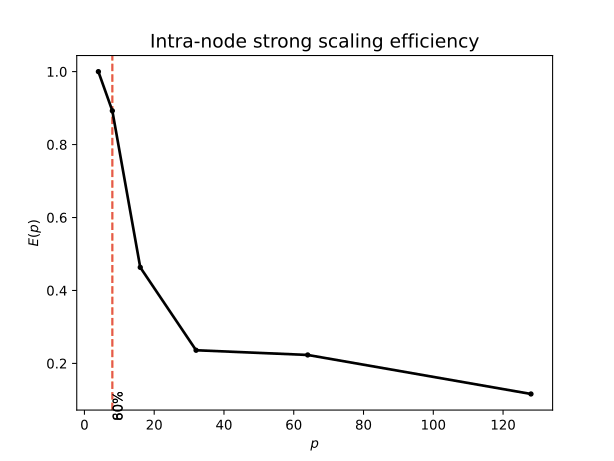
For a basic high-level analysis of intranode performance, we perform a strong scaling by fixing the problem size and increasing core allocation.

For this code, we tested with core counts in powers of 2 from 4 to 128 because the minimum number of cores HemeLB can use is 3.

Thread count	Time (s)	Parallel efficiency
4	3310.983	1.000
8	1854.760	0.893
16	1786.564	0.463
32	1753.458	0.236
64	927.553	0.223
128	891.100	0.116

Hence, our 80% threshold is at 8 cores and our 60% threshold is at 8 cores. As a proportion of the number of cores available, which is 128 on the node this was run on, this gives a score of 0.0625 and 0.0625.

Summary

The following table collates the results of all above sections. These scores are indicative only, and cannot truly be compared to one another meaningfully without taking into account domain knowledge and methodological differences between them.

Result	Score	Metric result
CPU	0.026955838	238.7050 MFLOP/s
IO	0.991235906	2.059562s
Intranode (80%)	0.0625	8 cores

In summary we can see that the I/O performance is extremely good, as the benchmark spends the vast majority of its time in computation. However, the core and intranode performance are considerably lower. Again the intranode scaling was performed relative to a 4 core run, rather than a serial run as is typical, though the single node scaling still drops off very rapidly. From the performance data listed on the UKRI Living Benchmarks page, we can see the indicative run is a whole 128 core node on COSMA. Therefore we do not have currently have access to any other intranode results for HemeLB, so further analysis is required.

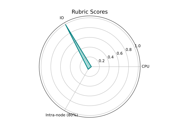
Following this high-level assessment, it is recommended that both the core and intranode performance are investigated in depth. Similarly, the GPU version of HemeLB must be analysed to study more compute rate that this benchmark can extract on a GPU. Finally, a internode analysis in the near future would be very interesting as HemeLB appears to focus on beyond single node scaling.

Trace analysis of HemeLB benchmark

Following from the high-level analysis we found a low intra-node metric and we want to dig into the parallelism of a node-level job. Here we have produced an instrumented binary with Score-P and then produced an automated trace analysis via Scalasca, using the Cube GUI for data visualisation and further analyses.

Time

First, we look at the break down of runtime (see table below) and find that the majority of time is in computation, though the MPI time is not insignificant.

	s (%)
Computation	2.22e4 (72.45%)
MPI	8444.54 (27.55%)

Computation

We use Cube to expand the call tree to mark the functions that constitute the largest proportions of runtime. We list below the functions that contribute most of the computation time.

Name	s (%)
void PreReceive()	1.62e4 (72.97%)
void PreSend()	3620.19 (16.30%)
void PostReceive()	1110.57 (5.00%)

Here void PreReceive() is by far the largest contributor to computation time. The functions appear close together in the call tree. With these functions in mind, we next turn to the MPI time.

MPI

Using Cube to expand the call tree again we find that the MPI time is dominated by a MPI_Waitall which is called for 7576.80s (89.72% of the MPI time). After this MPI_Waitall the next largest MPI routine is void Initialise() though in comparison this is only called for 433.50s (5.13% of the MPI time).

We can break this down further as of the 8444.54s of MPI routines, 7887.31s are spent in communication, in particular 7821.67s in point-to-point communcations, with 98.48% of this from the MPI_Waitall. In fact we find that 475.49s are due to Late Senders with the majority (85.60%) of these late senders resulting from this MPI_Waitall so this really seems to imply an issue causing excessive waiting times.

Delay costs

Moving to our next metric: delay costs, which highlights time spent from wait states. For this application the time spent is 548.52s which are further broken down in the table below.

Name	s (%)
SimulationMaster(...)	172.19s (31.39%)
void PreReceive()	149.81s (27.31%)
MPI_Waitall	135.53 (24.71%)
void PreSend()	58.16s (10.60%)
PostReceive()	17.74s (3.23%)

All of these functions showed up in the initial runtime metrics above, except for SimulationMaster(...), so these other routines are definitely causing excessive time from wait states. However, the SimulationMaster(...) only contributes 2.41% of runtime which is extremely small so we neglect this for now.

All of these delay costs are the result of MPI here and again overwhelmingly from point-to-point communications (91.96%), with late senders once again showing up as the main culprit at 475.27s (86.65%) of these delay costs. It seems that these main receive and send functions, along side the MPI_Waitall, are contributing the most to waiting.

Critical path

Our final review of the impact of these functions is on the critical path, which specifies the path through the runtime with no wait states, or in other words, represents the limitations on the total benchmark runtime. Here the critical path is 239.64s with same culprits appearing again

Name	s (%)
void PreReceive()	140.20s (58.50%)
MPI_Waitall	41.07 (17.14%)
void PreSend()	33.30s (13.90%)
PostReceive()	7.32s (3.05%)

With 9.28% of this attributed to imbalance, again largely concentrated in void PreReceive() and void PreSend().

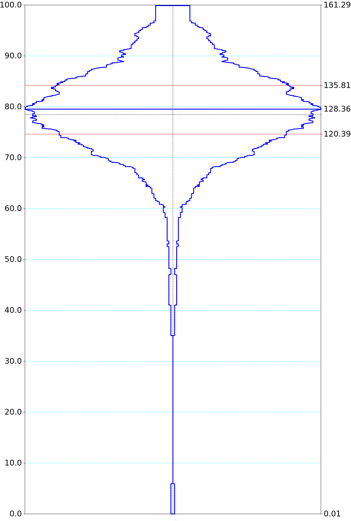
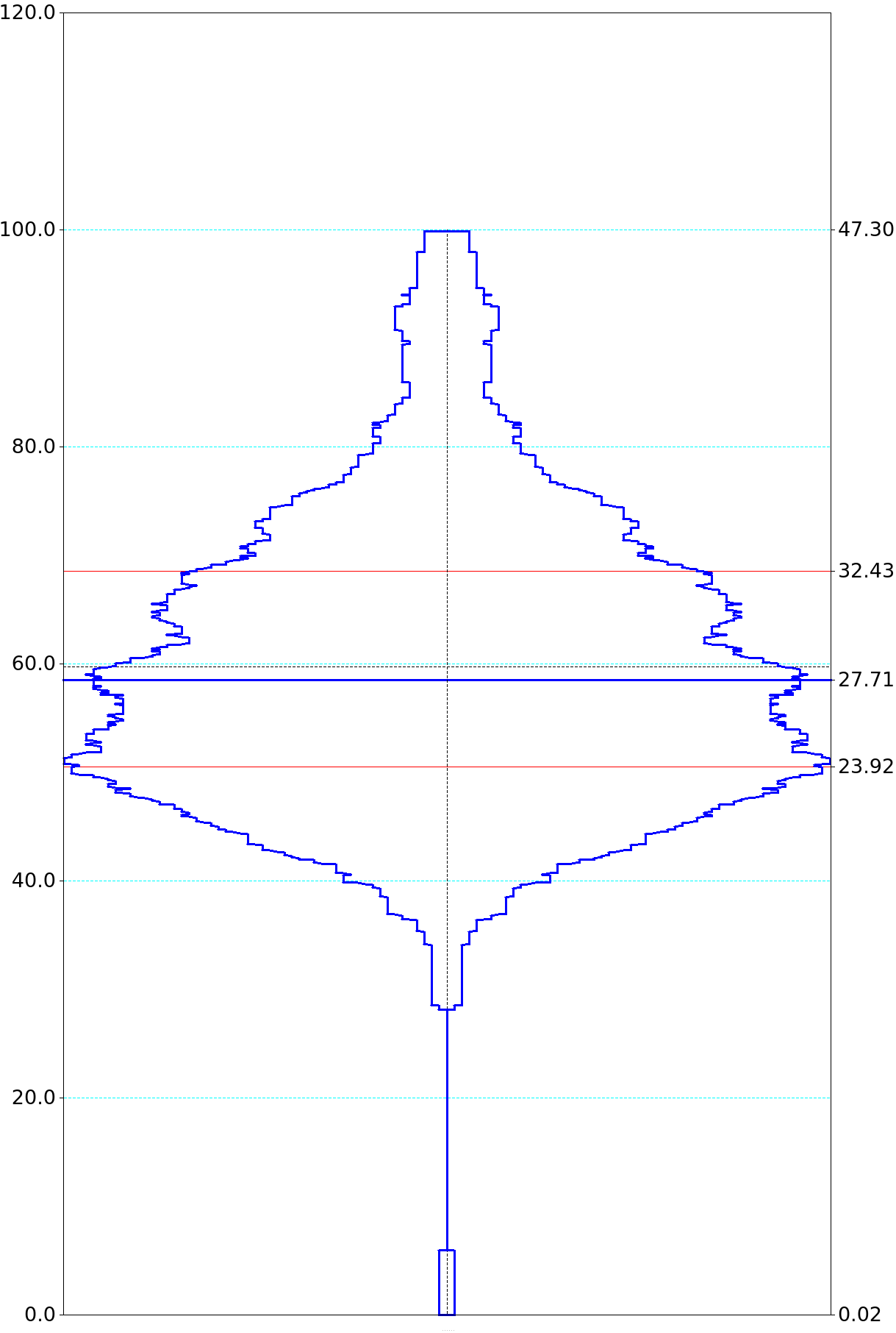
Time imbalances across ranks

The figures below show the distribution of the computation time across the 128 ranks for PreReceive() (top left), PreSend() (top right), MPI_Waitall (bottom left) and PostReceive() (bottom right). Across all four figures we do see evidence of imbalance.

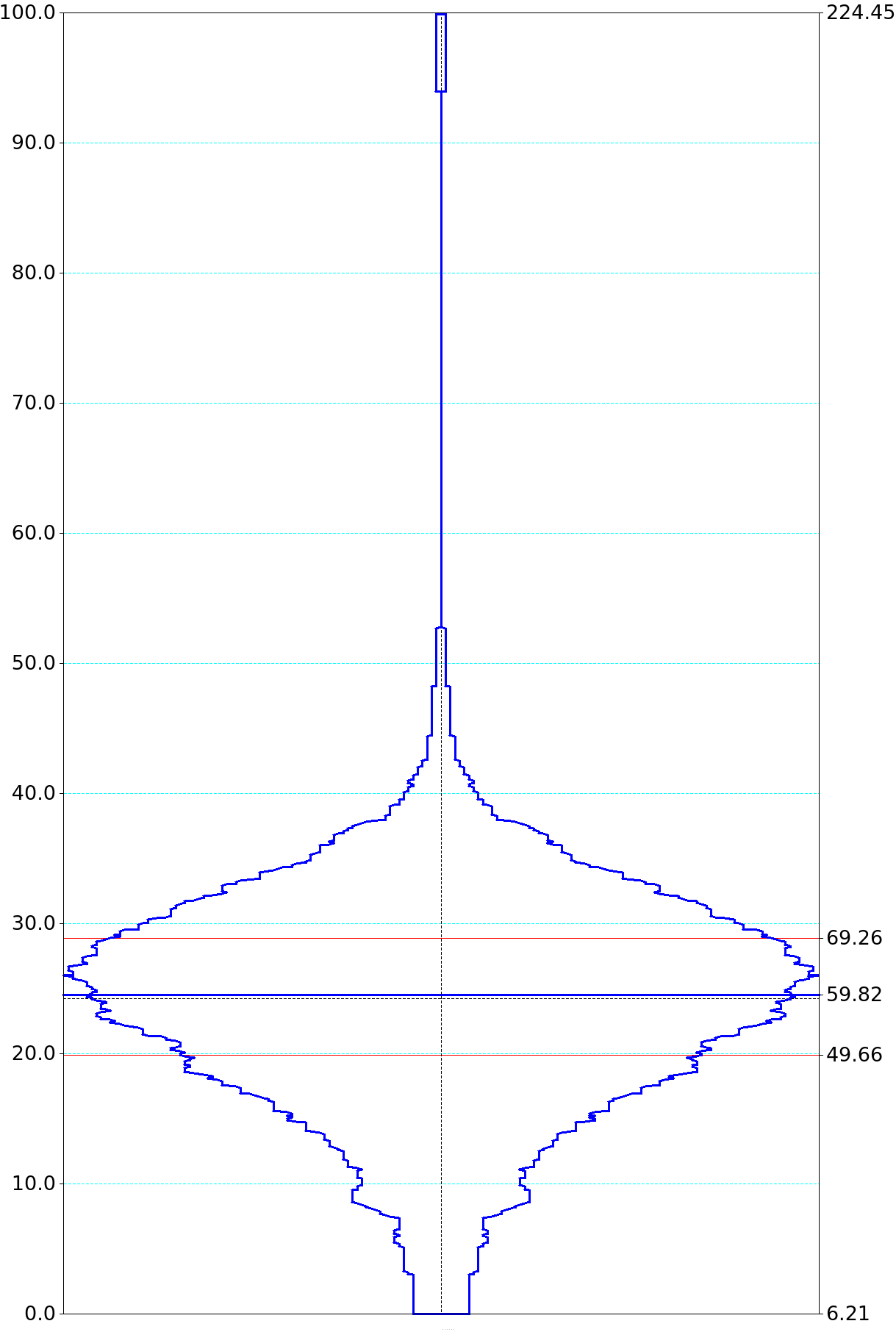
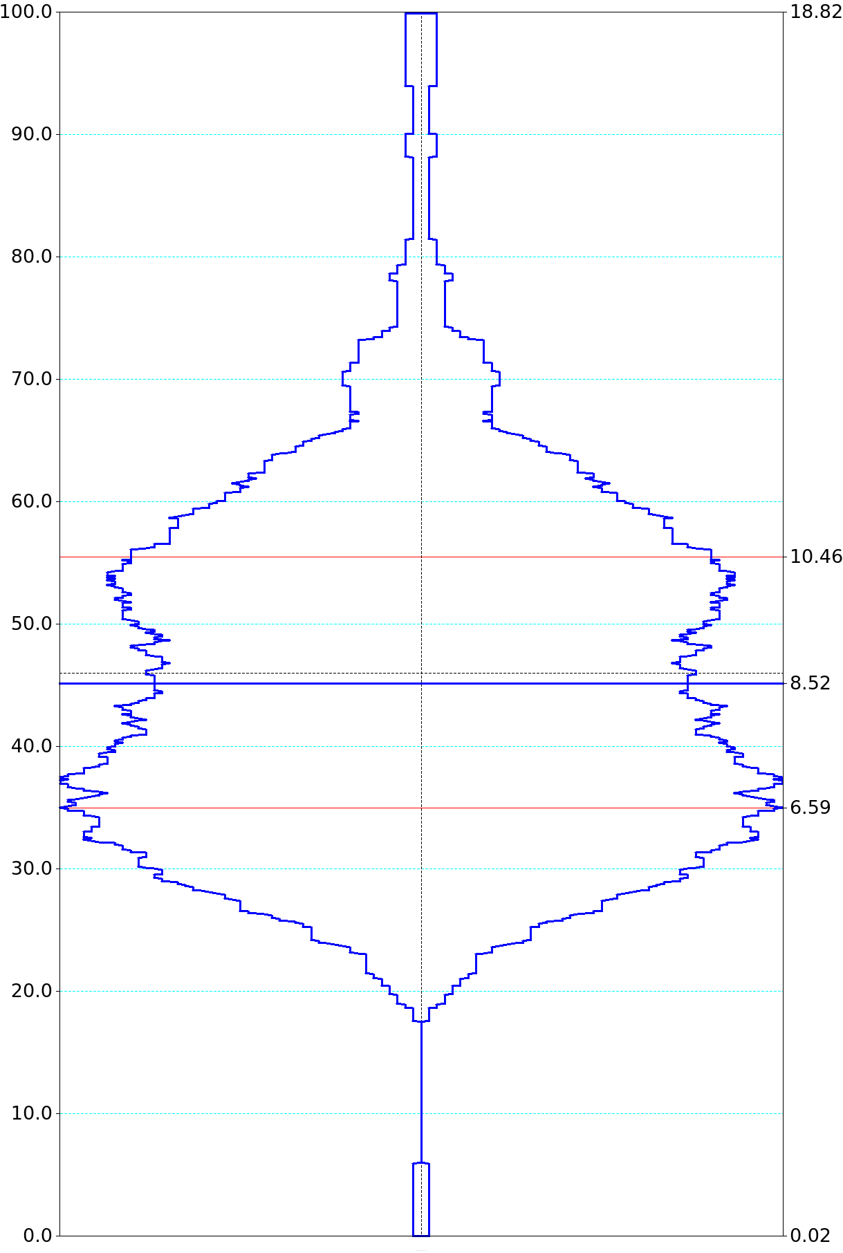
Computational imbalance

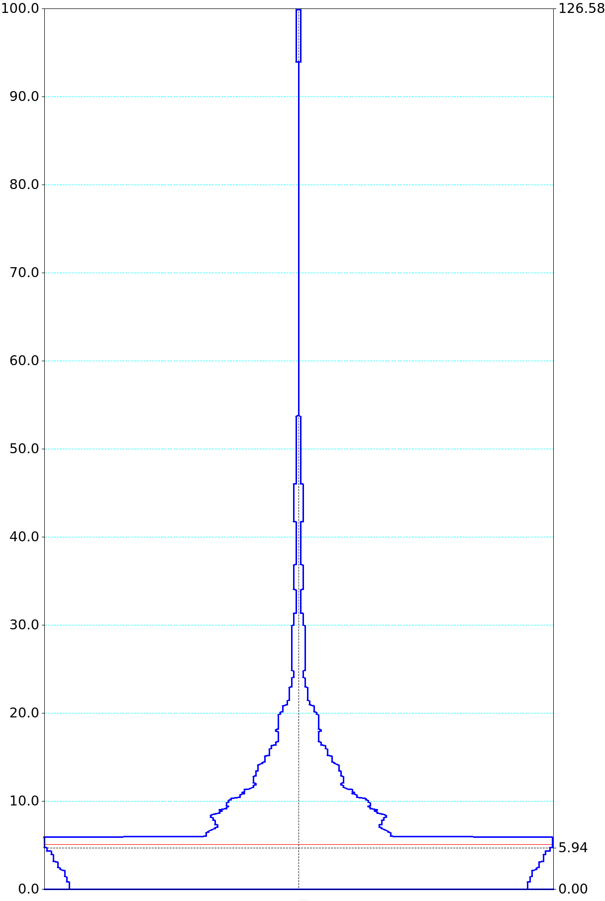
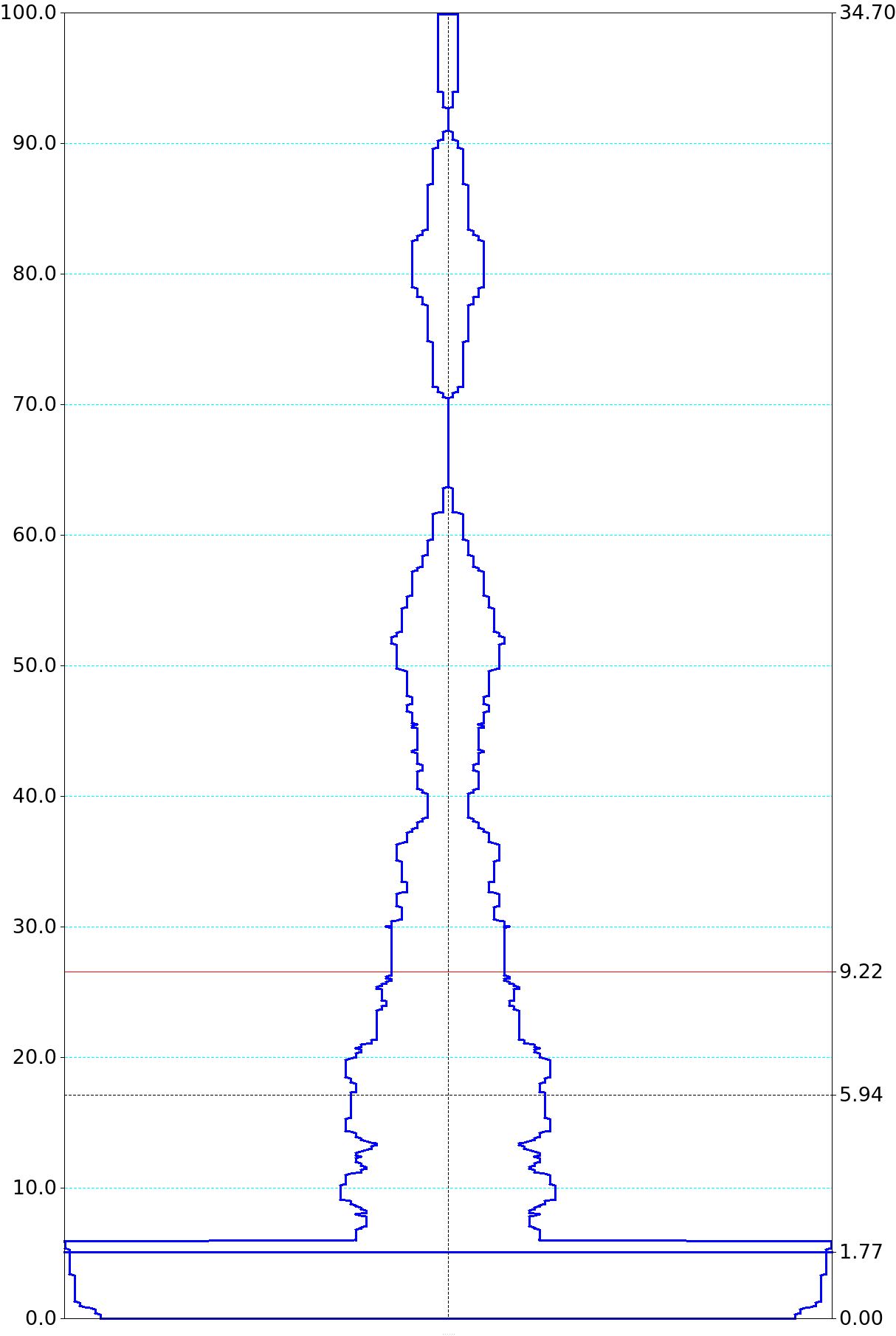
If we focus on PreReceive as the main culprit of computational imbalance, we can see how much of this computational is due to computational underload (left figure below) and overleaf (right figure below). At first glance that does seem to be evidence of some ranks being computationally overloaded.

Performance impact

We have found that there is evidence of imbalance in compute kernels. These kernels appear to precede the MPI_Waitall(). We find that 90.24% of performance impact is from functions on the critical path. Of these void PreReceive() contributed 59.20%. Hence, including this and the MPI_Waitall, contributes 77.56% to performance impact on the critical path. These are routines in which optimisations could effect the critical path and hence the programs runtime.

Summary

There is evidence of load imbalance in three kernels which appears to contribute to MPI late senders, which in turn are causing excessive wait times at an MPI_Waitall. Having quickly reviewed the source code for these kernels, it is clear they are responsible for Lattice Boltzmann steps around the MPI communications for lattice sites.

Two future steps could be taken:

1. Repeat similar analyses as part of a scaling run to see how this imbalancing varies with process count, though it should be noted that this is resource intensive.
2. Return to code owners to discuss the observed load imbalance to discuss how the work is divided across MPI ranks as this might direct subsequent analyses.