LAMMPS assessment (SHAREing)
Objective of preassessment
A test submission of LAMMPS, available at LAMMPS website and LAMMPS Github version tested Stable Release 22 July 2025, Update 3.
Disclaimer for testing
This is not a commentary on code quality, but an indicator of the quality of the current SHAREing testing methodology as of this date,
Disclaimer for assessment
This forms only a preliminary assessment of submission suitability and does not guarantee a full assessment. The preassessment will be provided to the submitter with information on how to continue to assessment or rejection.
Section 3.1, Benchmark setup
- Provide commands to fetch and build program, e.g.
git clone https://github.com/lammps/lammps mylammps
cd mylammps
module load gcc/15.2 openmpi cuda
cmake -Scmake -Bbuild -D PKG_GPU=on -D BUILD_MPI=yes
cmake --build build
mpirun -np 16 ./build/lmp -in bench/in.lj
The build process fails if there is a parenthesis in the directory name.
- Provide commands to fetch benchmark, unless provded directly by submitter, in which case attach with this document.
git clone <benchmark repository>
- Provide instructions on how to run the benchmark and the expected output, e.g. from lammps directory for fixed size runs; ```bash cd bench mpirun -np 8 lmp_mpi -in (in.lj,in.chain,in.eam,in.chute, in.rhodo)
from lammps directory for scaled size runs;
```bash
cd bench
mpirun -np 16 lmp_mpi -var x 2 -var y 2 -var z 4 -in (in.lj,in.chain.scaled,in.eam,in.chute.scaled, in.rhodo.scaled)
Scaling the variables xx, yy, zz and run in the in.lj benchmark.
This problem has greater than linear scaling in xx etc, and approximately linear scaling with “run”
Strong and Weak scaling is presented at the LAMMPS Benchmark site
- If there is existing scaling information (graphs or raw data) available attach the data to this report and add links here.
2 Description of working environment
1. Hamilton/Bede
    a. `multi` queue for requestng whole nodes (to reduce timing noise from other programs)
    b. Limit is likely to be of order 512 processors (see Section 3.1
2. Assessment tools
    a. High level assessment
            i. wall time
    b. low level assessment (requires privileges on host) *TODO*
        i.CPU wait time (for I/O / heterogenous compute)
        ii.cache
        iii.memory accesses
        iv. LIKWID to access performance counters, topology etc.
3 Compiler Setup
Cmake uses performant settings of the major compilers.
4. I/O
Minimal I/O and only summary writing to stdout at the end of the benchmarks is present.
3.5 Hardware information
AMD EPYC 7702 64-Core Processor on 1 node - Hamilton.
processor       : 64 per socket
model name      : AMD EPYC 7702 64-Core Processor
cache size      : 512 KB

MemTotal:       263152912 kB   #~250GB per node
MemFree:        256995420 kB
MemAvailable:   258291956 kB
3.7 Code separation
N/A
3.8 Historic optimisations
N/A
Report
from topics.core import core_perf
from topics.intra_node import intra_node_perf
from topics.inter_node import inter_node_perf
from topics.gpu import gpu_perf
from topics.io import io_perf
from topics.summary import summary_perf
Core
For a high-level core analysis we just want 2 measurements for a serial code:
- Maximum peak performance (Mflops/s)
- Measured average peak FLOPS (Mflops/s)
FLOPS
To measure these we use LIKWID, i.e., for FLOPS we use
likwid-bench -t peakflops -W S0:16kB:1
likwid-perfctr -f -C 0 -g FLOPS_DP ./my_exe
in which the input data for the peakflops microbenchmark is half the L1 cache.
# Target peak per core (Mflops/s)
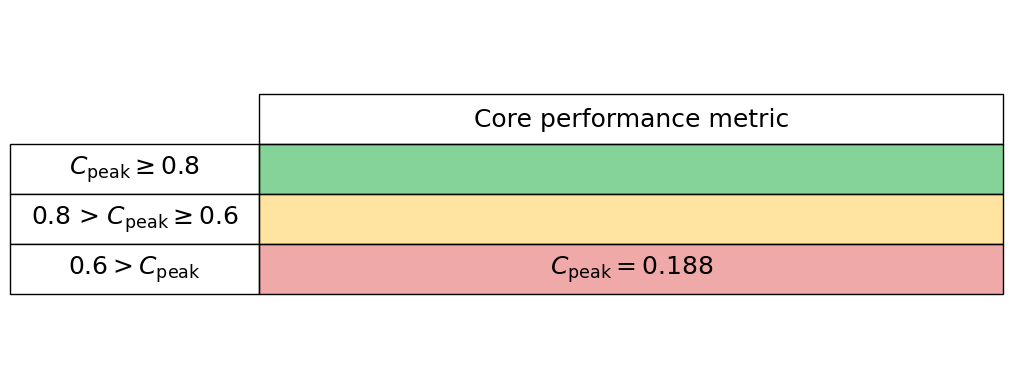
maximum_performance = 8808.70
# Measured average application peak (Mflops/s)
measured_performance = 1652.9897
We read these values into our core_perf class
core_performance_stats = core_perf(maximum_performance, measured_performance)
Generate the core performance table below
core_performance_stats.core_perf_table()
Intra-node
To quantify intra-node performance at a high level we reply simply on runtimes under a strong scaling analysis.
Serial run
If possible, we first measure the runtime of a serial application without any parallel libraries, e.g., compile without the -fopenmp flag. This can seem redundant but allows us to see the overhead of the parallel library when compared to a single-core run including the parallel library.
If the parallel library cannot be switched off simply, then we suggest just setting the serial runtime equal to a single-core (with parallel library enabled) runtime.
Strong scaling
We now perform a strong scaling analysis by keeping our problem sized fixed but increasing the core count up to the maximum for your hardware. For an OpenMP code the thread number can be set simply with the OMP_NUM_THREADS environment variable, however, with this method thread affinity can be an issue. It can make performance variable relative to a thread pinned run.
Thread pinning can be easily acheived by setting the OMP_PROC_BIND environment variable to close, however, we again make use of LIKWID
likwid-pin -c N:0-3 ./my_exe
This command can be nested into a for loop to increase the core count to efficiently perform a strong scaling analysis.
Input data
In the cell below we ask for the:
- Serial runtime
- A list of the core numbers used for the strong scaling
- A list of the relative runtime per number of cores
# Enter serial performance time (s)
import numpy as np
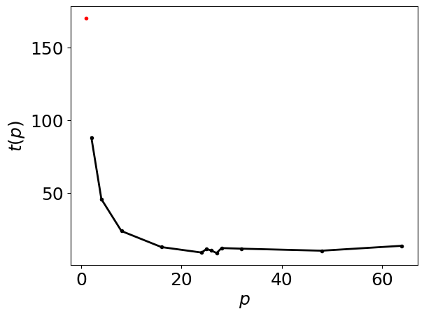
serial_time = 170.296
data = np.array([(64,13.5067),(48,10.1271),(32,11.5176),(28,11.9462),(27,8.52),(26,10.1898),(25,11.3001),(24,8.85465),(16,12.6093),(8,23.6582),(4, 45.6237),(2,88.0192 )
],dtype=[('Core count', 'i4'),('Loop Time','f4')])
# enter number of cores in each trial
number_of_cores = data['Core count']
# Enter time for each number of cores (s)
time = data['Loop Time']
We read these values into our intra_node_perf class
intra_node_performance_stats= intra_node_perf(serial_time, number_of_cores, time)
[0.19700409 0.35033063 0.46205375 0.50911587 0.74028863 0.64278456
 0.60281235 0.80134924 0.84409922 0.89977264 0.93315542 0.96737987]
[27 26 25]
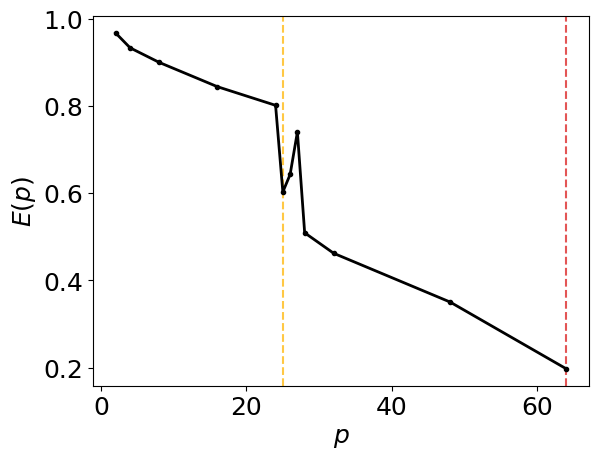
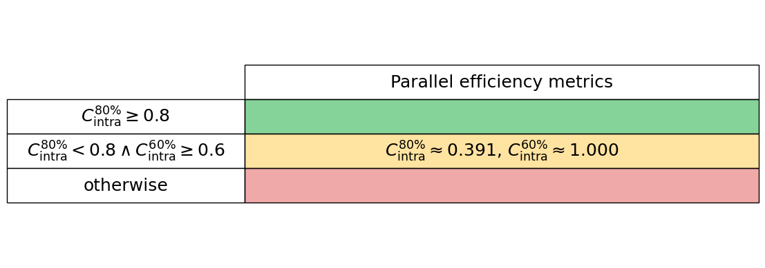
Generate the intra-node parallel efficiency plot below, including amber and red vertical lines which indicate the core counts below which the parallel efficiency drops to 80% and 60%, respectively.
intra_node_performance_stats.parallel_efficiency_figure()
Generate the intra-node runtimes plot below
intra_node_performance_stats.runtimes_figure()
Generate the intra-node performance table below
intra_node_performance_stats.intra_node_perf_table()
GPU
To quantify GPU performance at a high level we use two metrics:
- GPU utilisation or occupancy
- GPU memory usage
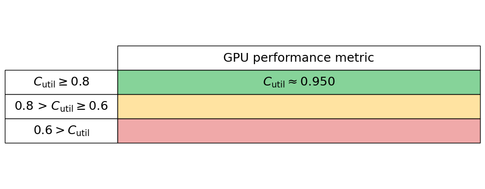
GPU utilisation or occupancy
This metric is typically a measure of the proportion of computational resources in use by the code. In Nvidia language this will likely be the proportion of streaming multiprocessors in use. We simply read this metric into our gpu_perf class below, and most GPU vendor’s tools will give this high-level metric for their hardware.
GPU memory usage
We compute the proportion of the maximum memory footprint used by the software by reading the theoretical gpu_peak_memory (typically from the vendor’s data sheets) and measure the actual memory usage, gpu_measured_memory, which again is typically given from most vendor tools.
gpu_utilisation = 0.95
We read these values into our gpu_perf class
gpu_performance_stats = gpu_perf(gpu_utilisation)
Generate the GPU performance table below
gpu_performance_stats.gpu_perf_table()
I/O
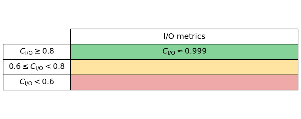
To quantify I/O (Input/Output) performance at a high level we simply ask what proportion of an applications total runtime is spent in read and writes. Many performance tools can give these high-level metrics, e.g., Intel VTune and Linaro Performance Reports. Typically these measures are given for both reads and writes separately, so we here read these two proportions in independently, thus the performance is charactertised by $C_{\mathrm{I/O}} = 1 - (C_{\mathrm{read}} + C_{\mathrm{write}})$. Therefore a low $C_{\mathrm{I/O}}$ value implies that the application is spending significant time in reading and writing to disk.
read_proportion = 0.00
write_proportion = 0.001
We read these values into our io_perf class
io_performance_stats = io_perf(write_proportion, read_proportion)
Generate the I/O performance table below
io_performance_stats.io_perf_table()