ExaGRyPE Performance Report
A test submission for the performance assessment of ExaGRyPE, available as part of the Peano repository under the stable branch p4. Pre-assessment was completed on 27-04-2026, and high-level assessment on 22-05-2026.
Disclaimers
- This report is not a commentary on code quality, but an indicator of the quality of the current SHAREing testing methodology as of 07-04-2026.
- The pre-assessment is only a preliminary assessment of submission suitability and does not guarantee a full assessment. It will be provided to the submitter indicating if the full assessment will be undertaken or detail reasons for rejection.
Table of contents
- 1: Benchmark setup
- 2: Description of working environment
- 3: Compilation and optimisations
- 4: Runtime behaviour, memory, storage and I/O
- 5: Computational complexity and scaling
- 6: High-level assessment
1: Benchmark setup
Fetch and build program
The main codebase, Peano, that ExaGRyPE is a part of, can be cloned using:
git clone -b p4 https://gitlab.lrz.de/hpcsoftware/Peano.git
The submitter specifies the version on the p4 branch (which is stable) must be used. To compile Peano, the submitter provided the following instructions:
libtoolize; aclocal; autoconf; autoheader; cp src/config.h.in .

automake --add-missing

./configure CXX=icpx CC=icx CXXFLAGS="-O3 -std=c++20 -xHost -fiopenmp -fsycl -Wno-unknown-attributes -Wno-gcc-compat" LDFLAGS="-fiopenmp -fsycl" LIBS="-ltbb" --enable-particles --enable-exahype --enable-blockstructured --with-multithreading=omp --enable-loadbalancing --with-mpi=mpicxx

make
Fetch and run benchmark
The benchmark itself is part of the codebase and can be accessed, compiled and run using:
cd benchmarks/exahype2/ccz4/single-black-hole

export PYTHONPATH=../../../../python:../../../../applications/exahype2/ccz4

python3 performance-studies.py -s fv-6 -et 1e-2 --plot 0.0 --cell-size 1.8 --trees 32 --scheduler native --output test

./test
The submitter has confirmed that the benchmark should take approximately 10 minutes to run. The regions of interest in the output can be identified as follows (comments starting with // are quotes from the submitter explaining each section):
// Calculation starts as the code plots start
AlgorithmicStep [TimeStep]

//The quantity of interest is the actual solve phase which is plotted eventually as
time stepping: 85.1353s (avg=17.0271,#measurements=5,max=23.0463(value #0),min=5.28955(value #3)
The parameter of interest to vary in the benchmark is --cell-size. This varies the number of cells value which can be read from the output with the following format:
27 tree(s): (#0:53/390)(#1:53/390)(#2:105/754)(#3:53/390)(#4:105/754)(#5:261/1534)(#6:105/754)(#7:53/390)(#8:105/754)(#9:53/390)(#10:105/754) (#11:261/1534)(#12:105/754)(#13:261/1534)(#14:20229/3250)(#15:261/1534)(#16:105/754)(#17:261/1534)(#18:105/754)(#19:53/390)(#20:105/754) (#21:53/390)(#22:105/754)(#23:261/1534)(#24:105/754)(#25:53/390)(#26:105/754) total=23479/24622 (local/virtual)
Reference architecture
The submitter has provided the Hamilton supercomputer at Durham University as a reference hardware. The assessor is based at Durham University and used the same system for this pre-assessment.
2: Description of working environment
Hardware information
The hardware details for Hamilton are available online. This information is corroborated by running cat /proc/cpuinfo and likwid-topology on one of the compute nodes via an interactive session on the test queue: srun -p test -N 1 --pty bash.
| Specification | Details |
|---|---|
| Number of compute nodes | Standard: 120; High-memory: 2 |
| Processors | 2 \(\times\) AMD EPYC 7702 64-Core Processors per node |
| Clock speed | 3.30 MHz per CPU |
| Sockets | 2 per node |
| Cores | 128 per node |
| RAM | Standard: 256 GB (246 GB available to users) per node; High-memory: 2 TB per node |
| Local storage | 400 GB SSD per node |
| NUMA domains | 8 per node (2 per socket), each with a dedicated memory channel and further split into 4 groups containing 4 cores each |
| Cache | 16 MB L3 cache per group, 512 KB of L2 cache per core and 32 KB of L1 cache per core |
Hamilton also has one GPU node with the following configuration (N.B. the assessor currently does not have access to this node and cannot corroborate the information):
| Specification | Details |
|---|---|
| Processors | 2 \(\times\) AMD EPYC 9555 64-Core Processors |
| GPUs | 8 \(\times\) NVIDIA H200 NVL |
| RAM | 2.2 TB |
| Local storage | 3 TB NVMe |
Job submission configurations
SLURM is used for job scheduling on compute nodes. The full list of options on Hamilton are provided in the online documentation for the cluster. The following configurations are relevant to this assessment to compile the code and run the executables, with values adjusted based on use case:
-p shared      # Or "multi" if using a full node
-t 01:00:00    # Jobs are not expected to take longer than an hour to run, but will be adjusted if needed
-n 2 -c 16     # Running on 32 cores, using 2 MPI ranks and 16 threads per rank
-N 1           # Using cores on the same node
--mem=16G      # Allocating 16 GB of RAM to the job
Libraries and modules
The system uses lmod to manage compute environments such as loading compilers etc. The documentation of the Peano codebase includes instructions for setting up the working environment on Hamilton:
module purge
module load oneapi/2025.2
export FLAVOUR_NOCONFLICT=1
module load gcc/15.2
module load tbb/2022.0
module load intelmpi/2021.16
export I_MPI_CXX=icpx
module load python/3.13.9
The environment setup is confirmed using module list:
Currently Loaded Modulefiles:
  1) oneapi/2025.2      2) gcc/15.2           3) tbb/2022.0         4) intelmpi/2021.16   5) python/3.13.9
Assessment tools
- Pre-assessment:
topandtimefor high-level wall time execution and memory usage analysiscat /proc/cpuinfoandlikwid-topologyfor hardware information
- High-level assessment:
likwid-benchandlikwid-perfctrfor measuring FLOPSlikwid-pinfor thread pinning to measure performance within and across NUMA domains
- Low-level assessment (may require admin privileges):
vtunefor detailed profiling and hardware metrics (especially for Intel systems and compilers)valgrindfor detailed memory analysismaqaoto identify opportunities for compiler optimisation
3: Compilation and optimisations
Hybrid: OpenMP + MPI configuration (as per submitter’s instructions)
The GNU Autotools build system (configure and make) is used for compilation. The submitter has included the -xHost flag to enable hardware-specific optimisations. The -03 optimisation flag ensures aggressive optimisation while complying with FP standards. The submitter has not reported any issues from these optimisations on the convergence and correctness of the results.
The code is compiled for the C++20 standard and using Intel compilers (icx and icpx). The submitter indicated a preference for the latest Intel compilers. On Hamilton, the latest compilers are a part of the Intel OneAPI 2025.2 suite which will be loaded with the recommended environment setup. Intel’s version of OpenMP is used with the -fiopenmp flag. GPUs are not enabled by default and would have to be enabled with a --with-gpu flag. But the submitter has indicated that they prefer the initial analysis to be done without GPUs. The submitter has stated further details on compilation flags can be found within Peano’s documentation.
The Peano codebase and the benchmark were compiled on a compute node via an interactive job with 8 GB of RAM and 32 threads, allocated on the same node: srun --mem=8G -c 32 -n 1 -N 1 -p shared -t 01:00:00 --pty bash. After loading the modules, Peano and the benchmark were compiled to create the test executable. To speed up the compilation, make was run with multi-threading using -j 32. The -g flag was also included to add debug symbols to the executable to enable the use of performance analysis tools during lower-level assessments.
The compilation of Peano completed successfully. For the benchmark compilation, the performance-studies.py Python script was also given the additional -j 32 parameter to limit the compilation to 32 threads (as it would attempt to compile over the whole node otherwise). However, the benchmark compilation resulted in errors due to some missing Python libraries. The assessor found the list of required libraries within the Peano documentation: jinja2, ast_comments and vtk and installed them in a virtual environment, after which the benchmark compilation ran successfully.
The executable was run after the compilation on the same interactive job. However, the run exited early with the following error:
Please verify that both the operating system and the processor support Intel(R) X87, CMOV, MMX, SSE, SSE2, SSE3, SSSE3, SSE4_1, SSE4_2, MOVBE, POPCNT, AVX, F16C, FMA, BMI, LZCNT, AVX2 and ADX instructions.
The assessor investigated this error and determined that the issue may be arising from the use of the -xHost flag which is meant to enable optimisations specific to the hardware, but may not be working correctly for the AMD processors on Hamilton. The performance assessment workbook also indicates that using -xHost on non-Intel hardware could result in unoptimised code. Furthermore, looking into compilation suggestions for Peano in its documentation, recommendations for DINE (which also has AMD processors) indicate using the -march=native flag instead of -xHost as the latter results in runtime issues. The assessor recompiled the codebase and benchmark, replacing -xHost with -march=native, which compiled successfully. The run of the updated test executable with the same configuration completed without any reported errors.
The compiled benchmark executable was re-named to test-base-omp-mpi to indicate its configuration.
OpenMP-only configuration
The submitter indicated that MPI usage could be turned off by removing the --with-mpi flag for ./configure. As an alternative option for the intra-node assessment requested by the submitter, another version of the Peano codebase and ExaGRyPE was compiled for an “OpenMP-only” configuration by removing the --with-mpi flag. The benchmark was also re-compiled using the performance-studies.py script for this configuration: test-base-omp-only.
Serial configuration
The serial configuration of the code is required for accurate speed-up analysis as \(t_{serial} \neq t_{p=1}\), where the latter is for a binary compiled for parallel runs. The serial version was compiled by removing both the --with-mpi and the --with-multithreading flags. The benchmark was also re-compiled using the performance-studies.py script for this configuration: test-base-serial.
GPU configuration
The submitter has indicated that GPU assessment is relevant for this codebase, but also stated that they are not pursuing it in this initial assessment.
For the sake of completeness, the assessor did attempt to compile the code on one of Hamilton’s GPU nodes, using information from the documentation on enabling GPU offloading and compiling for Grace Hopper testbeds. However, it was difficult to determine the right configuration, and all attempts resulted in compiler errors.
For follow-up assessments the assessor will liaise with the submitter to determine optimal compiler flags for GPU offloading on Hamilton.
4: Runtime behaviour, memory, storage and I/O
To analyse baseline behaviour, the benchmark (test-base-omp-mpi) was run on three configurations: single core (-n 1 -c 1), 32 threads on 1 MPI rank (-n 1 -c 32), and with 16 threads per rank on 2 MPI ranks (-n2 -c 16). Jobs were launched on compute nodes using a SLURM submission script per configuration. The submitter did not provide any information on the memory footprint of the benchmark, however, this was also not requested in the current version of the assessment form. The jobs were given access to 16 GB RAM as they only use a subset of a node’s resources.
The /usr/bin/time -v command was used to measure the execution time, and the sacct --format="MaxRSS" command was used to get memory usage statistics for the jobs after completion. For the latter, all configurations were run with mpirun to separate the memory usage of the actual job from resources used by the sbatch command. For the -n 2 -c 16 configuration, the maximum execution time between the 2 ranks is reported.
| MPI ranks | Threads per rank | Execution time (s) | Memory usage (GB) | Memory usage (%) | Lines of output |
|---|---|---|---|---|---|
| 1 | 1 | 244.62 | 7.02 | 44.25 | 193 |
| 1 | 32 | 56.94 | 0.440 | 71.25 | 399 |
| 2 | 16 | 46.46 | 3.00 | 3.90 | 399 |
The benchmark produced up to 400 lines of output, depending on the number of threads used. This included the lines reporting the value of interest i.e. number of cells indicated by the submitter, along with the processor ID, MPI rank ID and time step. All three configurations produced a total of 19683 cells by the end of the run (N.B. this value is lower than the expected 23479 cells indicated by the submitter). For the -n 2 -c 16 configuration, the trees built per rank had 19318 and 365 cells respectively at the end of the run.
Apart from the essential console output, the submitter had stated that unnecessary I/O (plots) can be switched off by providing the --plot 0.0 argument to performance-studies.py. The submitter has emphasized that using any other value for --plot enables the output. They also noted that the code neither reads nor writes to large input files. The assessor corroborates that the benchmark, which was compiled with --plot 0.0 as per the submitter’s instructions, did not write any files to storage not read any in.
5: Computational complexity and scaling
The maximum runtime of the benchmark, which is on a single core, is just over 4 minutes. Scaling the same job to 32 threads (or 2 MPI ranks with 16 threads each), which is a quarter of a node on Hamilton, already takes less than one minute, making a strong scaling analysis for the intra-node assessment on this job size difficult.
However, the submitter has indicated that the benchmark’s problem size should scale with the “number of cells” value. The primary problem size parameter to be varied is the --cell-size. In the example provided, this is set to 1.8. The submitter stated that this can be changed in multiples of three. Increasing the size of the parameter, for example to 5.4 leads to a smaller and coarser setup. The assessor tested this and with 5.4 (test-coarser-omp-mpi), the total number of cells generated were reduced to 729, taking only 12s on a single core. Conversely, running with --cell-size 0.6 (test-finer-omp-mpi) increased the number of cells generated to 514218, taking 744.52s to run. The latter case also increased the required memory to 200 GB, with all runs crashing due to out-of-memory errors with a 16 GB allocation. The --cell-size parameter can, therefore, be easily set for a sizeable benchmark for strong scaling and varied for weak scaling analysis. Furthermore, with a single core runtime of almost 20 minutes, the finer case can be used for strong scaling analysis.
The submitter has provided a link to detailed instructions and background information to the benchmark. This includes graphs detailing scaling in terms of load (number of cells and number of trees per rank) and runtime for two types of methodologies (regular grid and adaptive mesh). Explanations for each setting are also provided. Apart from --cell-size, the linked documentation lists other variable parameters that could impact the performance and scaling such as the type of solver used, the load balancing paradigm, task scheduling etc. The submitter has also indicated that they assume that a “one MPI rank per NUMA domain” configuration may be optimal and that there is “no restriction on GPU-MPI association”.
6: High-level assessment
The assessor was successfully able to compile and run the benchmark with multiple configurations. The problem size was also easy to scale and so the benchmark can be used for both strong and weak scaling analysis during the main analysis.
The assessor then proceeded with high-level assessment. The submitter had specified that out of the three performance dimensions, the ones relevant to this assessment and benchmark are:
Core-level assessment
For a high-level analysis of a single core’s performance, we look for the floating-point operation rate compared to the theoretical rate, \(R^{core}_{theoretical}\) for a core. The hardware capabilities were determined with likwid-bench pinned to a single core on the first socket of a node:
likwid-bench -t peakflops -w S0:16kB:1
To analyse the performance of a single core, the Serial version of the scaled “finer” benchmark (test-serial-finer) was run with likwid-perfctr to get the observed floating point rate
likwid-perfctr -f -C 0 -g FLOPS_DP ./test-serial-finer
Despite running on a single core, the job was given access to an exclusive node with all cores and 200 GB memory available to it. The observed and theoretical floating point rates were as follows:
| Rate | MFLOPS/s |
|---|---|
| \(R^{core}_{theoretrical}\) | 8883.75 |
| \(R^{core}_{observed}\) | 7028.03 |
Based on these results, we determined that this software has a score of \(C^{core} = \frac{R_{observed}}{R_{theoretical}}\approx 0.79111...\approx0.8\).
Intra-node assessment
As noted earlier, Peano and ExaGRyPE can be compiled and executed on a single node with one of two configurations. Both are analysed below using a strong scaling analysis over 1 to 128 cores, with the problem size fixed to the “finer” version of the benchmark (test-omp-only-finer). The Serial configuration was used to obtain the runtime of the 1 core/thread run.
OpenMP-only configuration
For thread/processor count (NUM_THREADS), likwid-pin was used to pin each OpenMP thread to consecutive logical cores on the node up till the number of threads used for that run:
/usr/bin/time -v likwid-pin -c N:0-${NUM_THREADS-1} ./test-omp-only-finer
All runs below were executed in the same SLURM job submission script which was allocated nodes on an entire core, and 200GB of memory:
#SBATCH -c 128       # Use all cores on the node
#SBATCH --mem=200G   # Memory allocated to the entire node
#SBATCH -N 1         # Run on an entire node
#SBATCH -p multi     # Use an exclusive node
However, for the run for 64 and 128 cores, the runs resulted in an out-of-memory error. They were run again on the bigmem partition, which allowed for increasing the memory size to 380 GB.
The table below shows the runtime and the parallel efficiency for the run per thread count. Alongside that, the maximum resident set size (MaxRSS) value tracked using /usr/bin/time -v also indicates the memory needs for each job.
| Threads (cores) | Time (s) | Parallel Efficiency | MaxRSS (GB) |
|---|---|---|---|
| 1 | 9255.00 | 1.00 | 186.54 |
| 2 | 5372.00 | 0.86 | 170.77 |
| 4 | 2536.52 | 0.91 | 171.60 |
| 8 | 1303.37 | 0.89 | 175.59 |
| 16 | 732.47 | 0.79 | 181.12 |
| 32 | 742.67 | 0.39 | 193.69 |
| 64 | 659.37 | 0.22 | 249.33 |
| 128 | 800.48 | 0.09 | 217.41 |
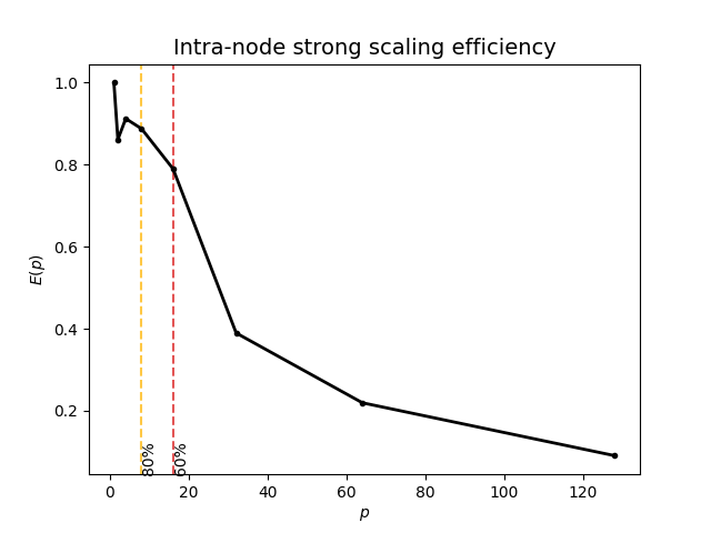
The graph above shows a steep decline in parallel efficiency as the number of thread were increased. The 80% threshold for the OpenMP version was determined to be at 8 cores and the 60% threshold at 16 cores: \(C^{80\%}_{intra(OpenMP)}=\frac{p^{80\%}_{critical,intra(OpenMP)}}{p_{max,intra(OpenMP)}}=\frac{8}{128}=6.25\%\) and \(C^{60\%}_{intra(OpenMP)}=\frac{p^{60\%}_{critical,intra(OpenMP)}}{p_{max,intra(OpenMP)}}=\frac{16}{128}=12.5\%\)
Hybrid (OpenMP + MPI) configuration
Based on the submitter’s indication that 1 rank per NUMA domain is expected to yield better performance, the Hybrid configuration (test-omp-mpi-finer) was run for each core count as follows with likwid-mpirun. An MPI rank was pinned to each of the 8 NUMA domains on the node, and consecutively allocating a thread to each of the 16 cores in the domain:
/usr/bin/time -v likwid-mpirun -n $MPI_RANKS -pin M0:0-15_M1:0-15_..._M${MPI_RANKS-1}:01-15 ./test-omp-mpi-finer
The runtimes up to 16 cores is similar to that of the OpenMP-only version, which was expected as they are run on a single rank. However, the runtimes for 32 to 128 cores were notably longer than the OpenMP-only version. Despite that, the change in parallel efficiency as the number of cores were increased for the Hybrid configuration is similar to that of the OpenMP-only version.
The memory usage of the benchmark was also tracked using /usr/bin/time/ -v. As observed in the table below, the memory footprint for all runs was much lower, and none of the jobs required the use of the bigmem partition.
| Rank | Thread per rank | Processors | Time (s) | Parallel Efficiency | MaxRSS (GB) |
|---|---|---|---|---|---|
| 1 | 1 | 1 | 9255.00 | 1.00 | 186.54 |
| 1 | 2 | 2 | 5420.00 | 0.85 | 0.02 |
| 1 | 4 | 4 | 2541.65 | 0.91 | 0.02 |
| 1 | 8 | 8 | 1317.85 | 0.88 | 0.02 |
| 1 | 16 | 16 | 744.52 | 0.78 | 0.02 |
| 2 | 16 | 32 | 1021.36 | 0.28 | 0.02 |
| 4 | 16 | 64 | 1056.50 | 0.14 | 0.02 |
| 8 | 16 | 128 | 1196.51 | 0.05 | 0.02 |
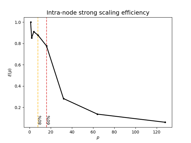
Like the OpenMP-only configuration, the 80% threshold for the Hybrid version is at 8 cores and the 60% threshold is at 16 cores: \(C^{80\%}_{intra(Hybrid)}=\frac{p^{80\%}_{critical,intra(Hybrid)}}{p_{max,intra(Hybrid)}}=\frac{8}{128}=6.25\%\) and \(C^{60\%}_{intra(OpenMP)}=\frac{p^{60\%}_{critical,intra(OpenMP)}}{p_{max,intra(OpenMP)}}=\frac{16}{128}=12.5\%\)
GPU/accelerator assessment
While GPU assessment was requested, as noted earlier, there was not enough information on GPU compilation for a system like Hamilton, and the instructions in the documentation for Grace Hoppers did not translate trivially to the H100s on it. The submitter had also noted that they are not pursuing the GPU analysis in the first run of this assessment. The GPU analysis was therefore not undertaken at this time.
Summary
The following table collates the results of all above sections. These scores are indicative only, and cannot truly be compared to one another meaningfully without taking into account domain knowledge and methodological differences between them.
| Result | Score | Metric result |
|---|---|---|
| CPU | 0.8 | 7028.03 MFLOPS/s |
| Intra-node OpenMP-only (80%) | 0.0625 | 8 cores |
| Intra-node MPI + OpenMP (80%) | 0.0625 | 8 cores |
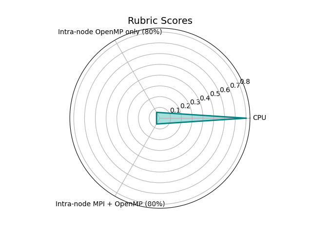
Drawing conclusions from each metric individually, the code’s core performance was determined to be good, and should not be the focus of further investigation.
However, the intra-node performance in both the OpenMP-only and Hybrid configurations shows poor strong scaling performance, albeit with better memory usage for the Hybrid one. The intra-node performance should be the initial focus of further lower-level analysis.